Used to describe where the central point of a given set of data lies compared to its extremes, the interquartile range is an essential component that is widely used in statistics. Classed as a form of statistical dispersion, it is also sometimes called the mid-spread or the H-spread. In this guide, you will find a thorough representation of how to calculate the interquartile range of a set of data, how to illustrate it, and discover some practical applications that it can be put to.
Definition: Interquartile range
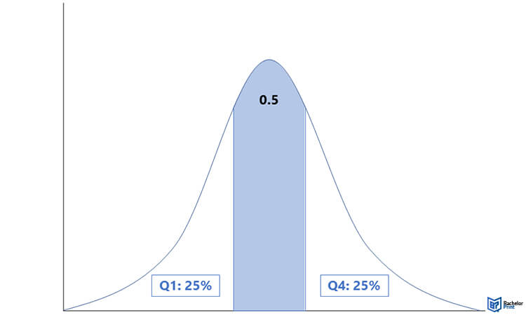
For a more profound understanding of the interquartile range, it is best to begin with a definition of what a quartile is. In statistics, a quartile defines a point when one-quarter of an ordered dataset is bounded. In other words, one quartile is at the 25% position, one is at the 50% position and the other lies at the 75% position.

Example
In a data set with 7 pieces of information, the lower quartile (Q1) would be in position 2 while the middle quartile (Q2) – also known as the median point – would be at position 5. Meanwhile, the third, upper quartile point (Q3) would be at position 6.
| Data set | 5, 11, 35, 37, 56, 89, 504 |
| Quartile | n/a, Q1, n/a, Q2, n/a, Q3, n/a |
In this example, the lower quartile is equivalent to 11 while the upper quartile is equivalent to 89. The middle quartile, or median, would be 37.
Therefore, the interquartile range would be the set of data between Q3 and Q1. Although the range of data in this example would be {35, 37 and 56}, the interquartile range would be the difference between Q3 and Q1, that is to say, a single figure only not a set. In the example given, this would be (89-11) = 78.
- ✓ Free express delivery
- ✓ Individual embossing
- ✓ Selection of high-quality bindings
Calculating the interquartile range
As the example above makes clear, the way to calculate the interquartile range (IQR) is to first work out what the upper quartile figure (Q3) is. Then, work out what the lower quartile figure (Q1) is. Simply take one from the other to give you the interquartile range. Therefore, the formula needed for this calculation is:
IQR = Q3 – Q1 or IQR = UQ – LQ
Q1 range – The lowest datum in the set through to the 25th percentile or ¼ of the data.
Q3 range – The datum from the 75th percentile of ¾ of the data through to the greatest datum in the set.
Simply put, the IQR is the difference between two quartile points bounding such ranges.
Interquartile range: Different methods
There are a number of methodologies that can be used for establishing the interquartile range. Let’s look at them systematically.
| The exclusive method | The inclusive method |
| The exclusive method excludes the median value from the IQR. It can be used for both even and odd-numbered data sets. | As the name suggests, the inclusive method includes the median value as part of the IQR calculation. It is typically used for odd-numbered data sets when the median can be found with ease. |
Interquartile range: Exclusive method
The exclusive method for calculating the IQR can be used for even and odd-numbered data sets. Here’s how you do each.
Data set with an even amount of data points
- Order the set from lowest to highest: {6, 10, 12, 15, 19, 21, 56, 57, 63, 70}.
- Find Q1 by taking the lower half of the set: {6, 10, 12, 15, 19}, and working out the middle value: 12.
- Find Q3 by taking the upper half of the set: {21, 56, 57, 63, 70}, and working out the middle value: 57.
- Since IQR = Q3 – Q1, the calculation to make is 57 – 12. Therefore, IQR = 45.
Data set with an odd amount of data points
- Order the set from lowest to highest: {6, 10, 12, 15, 19, 21, 56, 57, 63, 70, 75}.
- Now locate the median figure: The one in the middle which, in this case, would be 21.
- Find Q1 by taking the lower half of the set: {6, 10, 12, 15, 19}, and working out the middle value: 12.
- Find Q3 by taking the upper half of the set: {56, 57, 63, 70, 75}, and working out the middle value: 63.
- Since this is the exclusive method, the median value, 21, is excluded. As IQR = Q3 – Q1, the calculation to make is 63 – 12 = 51.
Interquartile range: Inclusive method
- Order the set from lowest to highest: {6, 10, 12, 15, 19, 21, 56, 57, 63, 70, 75}.
- Locate the median figure: The one in the middle, which, in this case, would be 21.
- Find Q1 by taking the lower half of the set but including the median figure: {6, 10, 12, 15, 19, 21}. In this case, Q1 would be the mean average of data points 3 and 4. The mean of 12 and 15 is (12+15) ÷ 2 = 13.5.
- Find Q3 by taking the upper half of the set but including the median figure: {21, 56, 57, 63, 70, 75}. In this case, Q3 would be the mean average of data points 3 and 4. The mean of 57 and 63 is (57+63) ÷ 2 = 60.
- IQR = Q3 – Q1 = (60 – 13.5) = 46.5.
When to use the interquartile range
The interquartile range is best used to avoid outlier results. When most figures are close to a central point but just a few would drastically adjust the mean average, for instance, viewing only the middle range of data can help to deal with errors or unlikely events.
Interquartile range graphical representation
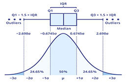
A boxplot, or a box-and-whisker plot as it is sometimes called, is used to summarize the interquartile range visually. It uses five pieces of information to help easily assess data sets. They show the lowest and highest values, the median and both the Q1 and Q3 points.
FAQs
This is the data point that lies 25% from the lowest point. Take the lower half of a set of data and work out the middle value.
This is the data point that lies 75% from the lowest point. Take the upper half of a set of data and work out the middle value.
This is the highest value in a set of data. It is not needed to work out the interquartile range, however.
Mathematicians don’t agree on whether the exclusive or inclusive method is best. There is no consensus.
