Simple linear regression is a key modelling method in statistics that represents the relationship between a dependent and independent variable. The regression shows the best fit straight line in a scatter plot, which depicts an equation that allows you to predict, diagnose, and interpret data outcomes. In sum, the aim is to assess the line that has the least distance from each data point in the plot. Simple linear regression is commonly used in fields like mathematics. engineering, and economics.
Definition: Simple linear regression
It is a statistical method used to model the linear relationship between two variables, where one variable (the dependent variable) is predicted or explained based on the other variable (the independent variable). The main goal of simple linear regression is to find the best-fitting straight line that can describe the relationship between the two variables and make predictions about the dependent variable based on the value of the independent variable.
Understanding simple linear regression
It is a statistical technique used to model the relationship between two variables. This section will discuss the advantages and disadvantages of using simple linear regression and its limitations.
Advantages of using a simple linear regression
- Provides a clear and concise relationship between the variables
- Can be used for prediction and forecasting
- Can identify outliers and influential observations
- Can be used to test hypotheses
- Simple to understand and implement
Disadvantages of using a simple linear regression
- Assumes linearity
- Assumes independence
- Sensitive to outliers
- Cannot establish causality
- Limited to one independent variable
Limitations
- Simple linear regression only applies when a linear relationship exists between the two studied variables. Other types of relationships cannot be modelled with this technique.
- It can only explain a portion of the variation in the dependent variable, and other factors may contribute to the variation that is not captured by the model.
- Its models are specific to the data from which they were derived and may not generalize well to other populations or contexts.
Assumptions of simple linear regression
There are three main assumptions of simple linear regression:
The relationship between the dependent and independent variables is linear. This means that the change in the dependent variable is directly proportional to the change in the independent variable.
The observations are independent of each other, meaning that the value of the dependent variable for one observation does not affect the value of the dependent variable for another observation.
The variance of the dependent variable is constant across all levels of the independent variable. The spread of the data points around the regression line is the same at all independent variable levels.
In addition to these three assumptions, another assumption of simple linear regression is:
Normality:
- The residuals (the difference between the observed and the predicted values) are normally distributed.
- This assumption is important because the residuals are used to estimate the standard error of the estimate.
Performing simple linear regression
The following section will discuss how to conduct a simple linear regression analysis.
Formula of the simple linear regression
The formula for simple linear regression is:
| The dependent variable | |
| The independent variable | |
| The y-intercept (when x = 0) | |
| The slope (the change in y) | |
| The error term (difference between the observed and predicted value of y) |
Simple linear regression in R
R is a programming language and software environment for statistical computing and graphics. It provides a wide variety of statistical and graphical techniques, including linear and nonlinear modelling , classical statistical tests, time-series analysis, classification, and clustering.
To demonstrate simple linear regression in R, we will use the mtcars dataset, which contains information about various cars, including their miles per gallon (mpg) and horsepower (hp).
To include this dataset in R, we can use the data() function:
data(mtcars)
Next, we can fit a simple linear regression model to predict mpg from hp using the lm() function:
r
model (less than symbol)- lm(mpg ~ hp, data = mtcars)
In this code, lm() stands for the linear model and mpg ~ hp specifies that we want to predict mpg using hp. The data = mtcars argument specifies that we are using the mtcars dataset.
Interpreting the results of simple linear regression
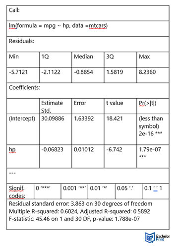
To view the results of the simple linear regression analysis in R, we can use the summary() function:
r
summary(model)
This will produce a table that looks like this:

When the results of a simple linear regression are put into a table by R, the table will typically include several rows of output. Here is an explanation of what each row means:
- The “Estimate” row displays the estimated value of the regression coefficient. This represents the change in the response variable for every one-unit increase in the predictor variable.
- The “Std. Error” row displays the standard error of the regression coefficient estimate. This measures the amount of variation in the regression coefficient estimate across different samples.
- The “t-value” row displays the test statistic for the hypothesis test of whether the regression coefficient is equal to zero. This is calculated by dividing the estimate by its standard error.
- The “Pr(>|t|)” row displays the p-value associated with the hypothesis test of whether the regression coefficient is equal to zero.
Presentation of the results
When presenting your findings, it’s important to provide the estimated effect (regression coefficient), standard error, and p-value. Additionally, it’s crucial to interpret the results in an easily understandable way to your audience. Our analysis revealed a significant correlation (p (less than symbol) 0.001) between education level and job satisfaction (R2 = 0.85 ± 0.011), indicating that for every increase of 2 years of education, job satisfaction increased by 0.85 units.
- ✓ Free express delivery
- ✓ Individual embossing
- ✓ Selection of high-quality bindings
Practical applications of simple linear regression
Simple linear regression is a statistical technique that can be applied to many practical situations, particularly those that involve understanding the relationship between two variables. In simple linear regression, one variable is considered the independent variable, while the other is considered the dependent variable.
One practical application of simple linear regression is in predicting the price of a house based on its size. In this case, the size of the house would be the independent variable, while the price of the house would be the dependent variable.
To calculate the simple linear regression for this situation, you would need to follow these steps:
-
Collect the data:
Measure the size of each house in square feet/meters and record the corresponding price of the house in your desired currency. -
Plot the data:
Create a scatter plot of the data, with the size of the house on the x-axis and the price of the house on the y-axis. -
Determine the regression line:
Draw a line of best fit through the data points on the scatter plot. This line should minimize the distance between each data point and the line. -
Calculate the slope and intercept:
Use (y = mx + b) to determine the slope (m) and intercept (b) of the regression line. The slope represents the change in price for each unit increase in size, the intercept represents the price of a size 0 house. -
Evaluate the regression line:
Check the goodness-of-fit of the regression line by calculating the correlation coefficient (r) and the coefficient of determination to indicate how well the regression line fits the data.
Once you have calculated the simple linear regression for this situation, you can use it to make predictions about the price of a house based on its size.
FAQs
Simple linear regression is a statistical method used to examine the relationship between two variables: a dependent variable and an independent variable.
The goal is to determine if there is a linear relationship between the two variables and to use this relationship to make predictions about the dependent variable based on the independent variable.
Simple linear regression examines the relationship between two variables, where one variable is the independent variable and the other is the dependent variable.
On the other hand, multiple linear regression involves examining the relationship between more than two variables, where one variable is still the dependent variable, but multiple independent variables may influence it.
The slope of the regression line represents the change in the dependent variable (y) for every one-unit increase in the independent variable (x).
- A positive slope indicates a positive relationship between the variables.
- A negative slope indicates a negative relationship.
The residual analysis involves examining the differences between the observed values of the dependent variable and the predicted values based on the regression line. It is used to assess the accuracy of the regression line and identify any outliers or influential observations that may be affecting the results.
