Skewness, a fundamental term in the realm of statistics, serves as a crucial measure of the asymmetry of a probability distribution. It provides significant insights into the shape of a dataset, specifically how it differs from a symmetric normal distribution. As we delve deeper into this statistical concept, we will explore its importance in data analysis, its calculation, and the types of skewness. Understanding skewness is an essential step towards comprehensively interpreting statistical data.
Definition: Skewness
Skewness is a distortion, bend, or asymmetry that moves away from a data set’s normal distribution or the symmetrical bell curve. This deviation may shift to the left or right of the symmetrical bell curve. Generally, the skew of a normal distribution is zero because it’s symmetrical on either side.
Types of skewness
Skewness impacts the string or tail of data points away from the median. The three types of skewness include positive, zero, and negative, as explained below:
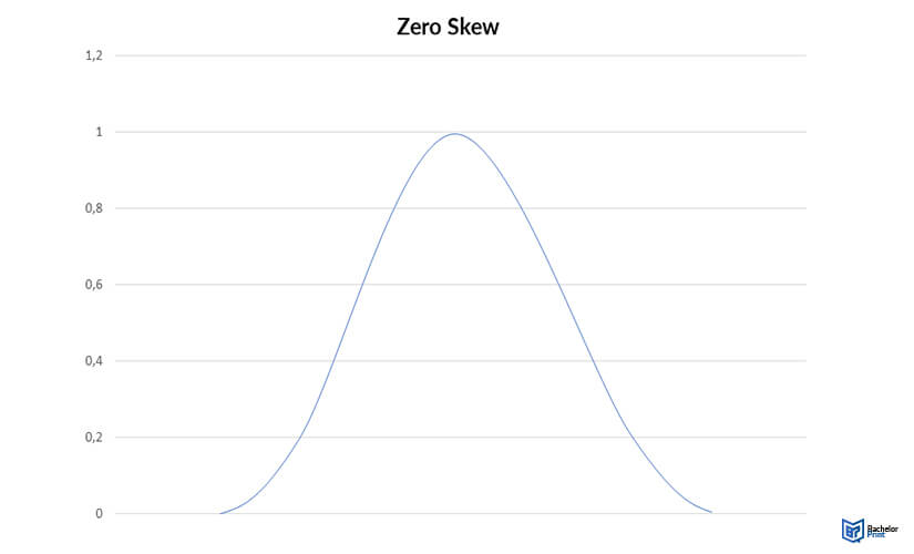
Zero skew
Normal distributions usually have zero skew values because the left and right sides are symmetrical. Other symmetrical distributions with a zero skew include some bimodal (two-peak) and uniform distributions.
The easiest way to know if variables are symmetrical is by using a histogram. If the distributions on both sides of the histogram are balanced, they have a zero skew. Additionally, a zero-skew distribution has an equal mean and median.
Zero skews: mean = median
Note that real-world data rarely have exact equal mean and median. However, if the median and mean are close to being asymmetrical, they have usually considered zero skews, for instance, a mean of 261.5g and a median of 285g.

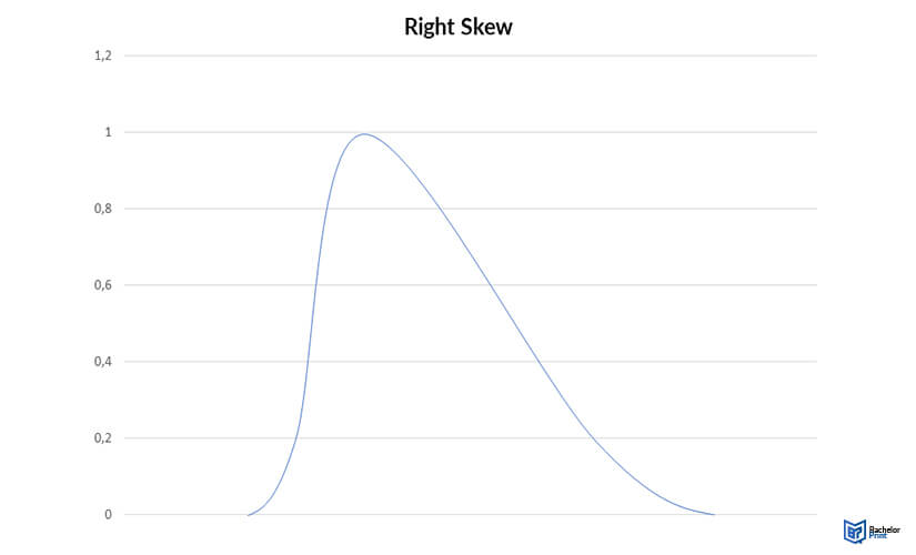
Right skew (positive skew)
A right-skewed distribution, also called a positive skew, has a longer tail on its right side. The mean of right-skewed data sets is greater than the corresponding median. This is because extreme values impact the mean more than the median.

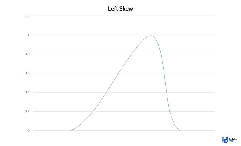
Left skew (negative skew)
A left-skewed distribution or a negative skew has a longer tail on its left side. Here, the mean is almost always lesser than the median.

How to calculate skewness
Pearson’s formula is the standard formula used to calculate skewness. This formula uses the theory that the mean and median in a skewed distribution are unequal, and it’s explained as follows:
Pearson’s median skewness:
3 × (mean-median)/standard deviation
This formula is essential for understanding the standard deviation values that separate the mean and median. In real-life observations, Pearson’s median skewness rarely has an exact score of zero. If your data results in a zero-skew score, consider it a zero-skew.
No standard convention counts as “close enough” to zero. However, some scholars concur that values of -0.4 and 0.4 are a reasonable cutoff for larger samples.
Skewness in data
Most statistical procedures assume that residuals or variables are normally distributed. You can use a skew to check whether your variables are appropriate for your statistical approach. You have the following three choices if you want a normal distribution, but you have skewed data:
Transformations based on the skew type
You can use the following transformations based on the skew type:
| Type of skew | Intensity of skew | Transformation |
| Right | Mild | Don't transform |
| Moderate | Square root | |
| Strong | Natural log | |
| Very strong | Log base 10 | |
| Left | Mild | Don't transform |
| Moderate | Reflect* square root | |
| Strong | Reflect* then natural log | |
| Very strong | Reflect* then log base 10 |
*The term “reflect” means you should take the greatest observation, K, before subtracting each observation from K+1. It would be best if you remembered that this observation changes the direction of variables and any relationship it has with other variables; such as, negative relationships become positive.
Example: Right-skewed variable transformation
You decide to perform a linear regression to predict the yearly number of sunspots. However, the results show that the data is not normally distributed. You discern that the sunspots observed yearly are right-skewed; hence, you can address this issue through a transformation.
You have another option, ignoring the skew because linear regression is not sensitive to skew. The first step is using a square root transformation. If this change isn’t enough, move to the next transformation step, as the table below shows:
| Number of sunspots per year | Sqrt (number of sunspots per year) |
| 23 | 4796 |
| 16 |
4000 |
| 11 |
3,317 |
| 5 | 2,236 |
The next step is placing your results in a histogram. If the skew is close to zero, replace the number of sunspots observed yearly with the transformed variables. Since the skew is near zero, likely, the linear regression is now normally distributed.
Printing Your Thesis With BachelorPrint
- High-quality bindings with customizable embossing
- 3D live preview to check your work before ordering
- Free express delivery
Configure your binding now!
FAQs
A value of between 0.5 and 1 or -0.5 and -1 means that you have a moderately skewed distribution. On the other hand, a highly uneven distribution has a skew value less than -1 or greater than 1.
Skewness shows you how much a variable differs from the normal distribution. In the real world, it’s beneficial in measuring performance and investment returns.
Any distribution with a negative skew is often less than zero and appears on the left side of the symmetric distribution.
Both these variables measure a distribution’s shape. Skewness measures a distribution’s asymmetry, while kurtosis measures how heavy a distribution’s tail is relative to the normal distribution.
