Degrees of freedom in statistics refer to the number of independent values that can vary in an analysis without breaching restrictions. This poses a key role in terms of determining accurate inferential statistics that impact a range of crucial distributions, such as a chi-square distribution, probability distribution, or linear regressions. Although degrees of freedom denote a subtle concept in data analysis, they are essential in drawing accurate critical values and statistical conclusions.
Definition: Degrees of freedom
Degrees of freedom represent the maximum quantities of independent observations and values that can be applied to statistical distributions without affecting any given limitations. They serve as tools to interpret precise estimates of statistical parameters or values of a sample size. There are test-specific formulas, depending on the distribution parameters that are anticipated. The classical formula for degrees of freedom for a one-sample t-test is as follows:
where,
-
= Degrees of freedom
-
= Sample size
The concept of degrees of freedom is specifically integral concerning statistical analysis and various statistical distributions like the chi-square distribution, probability distribution, t-distribution, and F-distribution. This is so, as the evaluated distribution parameters determine their shape and adjust their value points according to sample size. As a result, an accurate conclusion can be drawn from the inference about the sample size.
Note: Unlike the t-distribution, chi-square distribution, probability distribution, and F-distribution, a normal distribution is part of another family of distributions and thus, does not adjust according to the sample size. In other words, the correlation among observations stays constant regardless of the number of independent observations. Therefore, degrees of freedom are usually not a primary concern for normal distributions.
Example of degrees of freedom
Using a random sample, the following example outlines the process of calculating the sample variance considering degrees of freedom, with a dataset of five numbers. In evaluating sample variance, they are crucial, as we use a population nasty estimate instead of the true population nasty.
Firstly, we must calculate the sample nasty of the dataset, which defines the arithmetic nasty of the five values. For this, we use the formula of the sample nasty:
where,
-
= individual sample points
-
= sample size
-
= sample nasty
Then we implement the values into the formula.
As a second step, we calculate the squared deviation of each number in the dataset.
As a third step, all the squared deviations of each number should be added together.
In the fourth step, we insert the sample size of 5 into the degrees of freedom formula.
At the end of calculating the sample variance, we inserted the total number of items in the formula, which is minus the number of items in the dataset. In this example, only one parameter (the arithmetic nasty) was determined from the dataset, meaning that the number of independent values is reduced by one. Hence, the degrees of freedom are one less than the initial number of values.
In the last step, we ultimately calculate the sample variance by dividing the sum of squared deviations by the degrees of freedom.
Finding and applying df in statistics
Given a set of numbers, all numbers, except for one, are free to vary. This is always the case, as all numbers can be selected without any restrictions until one is left. The remaining number becomes dependent on the given average, meaning that it is no longer free to vary. In other words, at least one item in a set must conform to the given average.
Degrees of freedom take on the shape of the t-distribution when used in t-tests to assess the p-value. The shape of the t-distribution varies depending on the sample size. Determining them in statistics is integral to an array of aspects of data analysis, among others, in hypothesis testing, confidence interval, chi-square testing, variance, and regression analysis.
Calculating degrees of freedom
To calculate the degrees of freedom for statistical models and distributions, you must subtract the number of restricted values from the overall sample size. The constraints refer to parameters or critical values that are drawn from intermediate calculations of the statistic. Thus, they can’t be negative values and the number of parameters can’t exceed than the sample size. The intermediate calculations of the statistic typically entail test-specific formulas, depending on commonly used parameterized linear models or statistical distributions.
| Statistical test | Formula | Definition |
| One-sample t-test | Df = N - 1 | N = sample size |
| Two-sample t-test | Df = N1 + N2 - 2 | N1 = sample size of group 1 N2 = sample size of group 2 |
| Simple linear regression model | Df = N – (k + 1) | N = number of data points k = number of predictors |
| Chi-square goodness of fit test | Df = k – 1 | k = number of groups |
| Chi-square test of independence | Df = (r-1) x (c-1) | r = number of rows c = number of columns |
| One-way ANOVA between-group | Df = k - 1 | k = number of groups |
| One-way ANOVA within-group | Df = N - k | N = sum of all sample sizes k = number of groups |
Degrees of freedom in t-test
Applying the degrees of freedom in hypothesis testing can, for example, be done through t-tests. They are crucial in choosing the appropriate distribution for the test statistic and determining the critical values, which are compared with the test statistic. For t-tests, the critical values are commonly drawn from the t-table or calculated in software. Depending on the assessed values, the t-distribution will vary in shape, which is overall impacted by the sample size.
The following illustrates an example of using the t-test with two samples to evaluate the degrees of freedom.
For this, we insert the N values in the given degrees of freedom formula.
Then we insert the values into the formula to calculate the dfs.
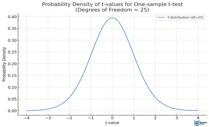
The y-axis of the graph below showcases the probability density of various t-values for a one-sample t-test with 25 degrees of freedom, while the x-axis depicts the likelihood of independent observations of each t-value under the null hypothesis.

Degrees of freedom in chi-square tests
Chi-square tests are one of the most powerful hypothesis tests. For this, the degrees of freedom are derived from the number of groups in the chi-square goodness of fit test. For the chi-square of independence test, we multiply the number of rows subtracted by one and the number of columns subtracted by one. To determine critical values of the chi-square distribution, you use the chi-square table. Based on the chi-square table, you can make a comparison between the observed values and the expected values under a certain hypothesis, as it contains realistic estimates of the degrees of freedom and the significance level.
The subsequent example illustrates how to calculate them in a chi-square test for independence on a contingency table.
For this, we insert the values into the given degrees of freedom formula.
Then we insert the values into the formula to calculate the dfs.
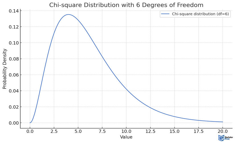
The y-axis represents the probability density of various values for the chi-square test with 6 degrees of freedom. The x-axis shows the values of the chi-square statistic.

Linear regression
In a linear regression, we need the number of data points and the number of estimated parameters to calculate the degrees of freedom. They define an essential concept for a linear regression model, as it refers to the number of independent parameter estimates in the model. Additionally, they assist in quantifying the extent of information used for the model’s parameter estimates against the amount of information that is left for estimating variability or errors.
The parameters of a simple linear regression typically lay at 2, one for the slope and one for the intercept. The following depicts an example using a simple linear regression for calculating the degrees of freedom.
For this, we plug in the values into the given degrees of freedom formula.
Then we insert the values into the formula to calculate the dfs.
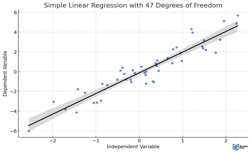
The following scatter plot graph shows the relationship between the independent and dependent variables of a simple linear regression with 47 degrees of freedom. The black line represents the best-fit linear regression.

One-way analysis of variance (ANOVA)
Under the null hypothesis in a single ticket ANOVA, you can conduct the F-test statistic. The F-test belongs to the most powerful hypothesis tests, serving as a tool to make a comparison between the variances of two or more populations. There are, essentially, two types of degrees of freedom that can be drawn from a single ticket ANOVA, between groups and within groups.
A single ticket ANOVA between groups (df1) evaluates the variability based on the interaction between populations. It’s evaluated considering the number of groups subtracted by one. On the other hand, a single ticket ANOVA within groups (df2) is associated with the variability within populations. Thus, it is calculated considering the total number of observations across groups subtracted by the number of groups.
For this, we plug in the values into the given degrees of freedom formula for df1 and df2.
By inserting the values into the given formula, we can calculate df1 as follows.
Next, we calculate df2 by using the respective formula.
At last, we calculate the dftotal by using the following formula.
Based on these df values, we can now compare them with a critical value from the F-distribution table to calculate the F-statistic for the ANOVA and determine its significance.
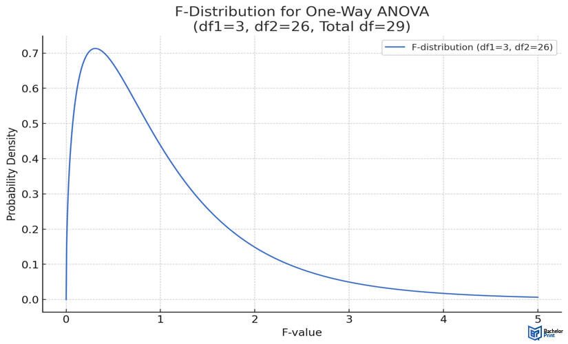
The graph below shows the F-values on the x-axis and the probability density on the y-axis to illustrate the F-distribution for a single ticket analysis of variance (ANOVA), where df1=3, df2=26, and dftotal=29.

- ✓ 3D live preview of your individual configuration
- ✓ Free express delivery for every single purchase
- ✓ Top-notch bindings with customised embossing

FAQs
The degrees of freedom in statistics, abbreviated “d.f.” or “df,” define values or variables in a data set that are free to vary. If they are equal to a lower number, the values, or variables are more restricted. They are vital in drawing accurate statistical conclusions.
This depends on the statistical test that is used to calculate the degrees of freedom. For instance, for the t-test with one sample, the degrees of freedom formula is N – 1, as only one parameter is estimated, whereas the t-test with two samples requires two estimated parameters, which is why the formula is N – 2.
Depending on the chosen intermediate statistical test, the formula for calculating and determining the degrees of freedom varies. The calculations through a t-test, chi-square test, simple linear regression, and single ticket ANOVA are outlined in the article.
Degrees of freedom primarily relate to the size of the sample; however, this is not always the case. The larger the degrees of freedom, it can be interpreted that the larger the given sample size. With a higher number of degrees of freedom, there is a higher chance to reject a null hypothesis that is inaccurate and, instead, draw a significant result.
Essentially, the degrees of freedom of an estimated parameter refer to the number of values that are free to vary or independent in a data set. These are typically calculated through intermediate statistical tests such as t-tests, chi-square tests, regression analyses, etc.
