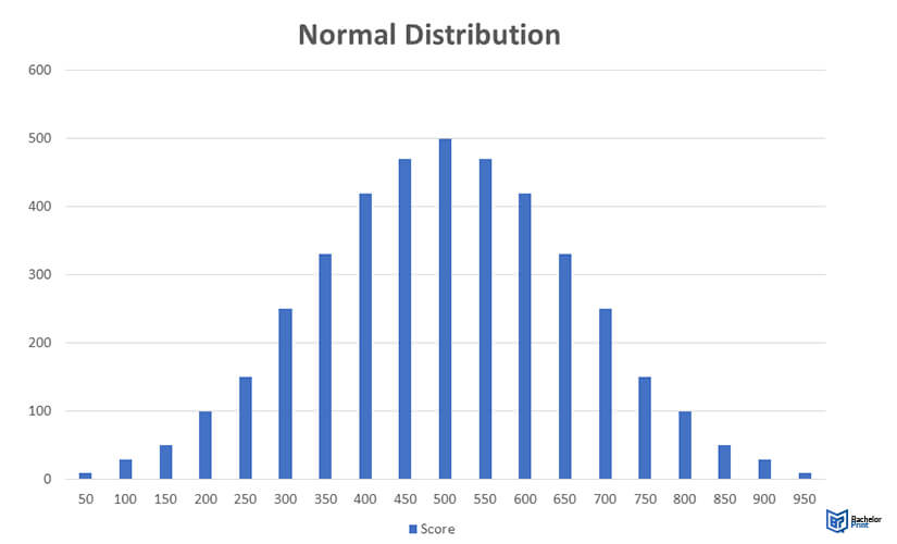
The normal distribution is a fundamental concept in statistics, defined by a symmetrical, bell-shaped curve that represents data clustering around a central mean. It describes numerous natural phenomena and underpins many statistical methodologies, making it indispensable for inferential statistics. This concept assists in understanding data variability, predicting outcomes, and testing hypotheses in diverse research fields.
Definition: Normal distribution
A normal distribution (Gaussian distribution) refers to a symmetrical probability distribution near the mean. Most observations, group around the peak and the probabilities of other values in the set lessen gradually in both directions.

The matter of normal distribution
Most variables used in scientific research display normal or near-normal distribution. Such variables include height, income, weight, literacy levels, and exam test scores. Since most of these variables display a normal distribution, many scientists use tests designed for normal distributions.
Knowing the characteristics of this distribution enables students and researchers to make verifiable conclusions and predictions from data samples representing larger populations. Such samples may be selected randomly or picked using the most representative elements of the population in inferential statistics.
The properties of normal distribution
The standard deviation and the mean are the two main parameters in a normally distributed data set:
- Mean – The mean is used as one of the main measures of central tendency in quantitative research. It is used in a distribution to define the peak, and most points tend to cluster around the mean.
- Standard deviation – It measures the variation of the distribution’s data points from the mean. The standard deviation illustrates how spread the data points are from the mean and is calculated by determining the square root of the variance.
Normal distributions exhibit the following characteristics:
- Symmetry – It assumes a symmetrical shape. This implies that the curve can be divided into two equal halves. The symmetrical shape of the distribution is because half of each observation falls on either side of the bell curve.
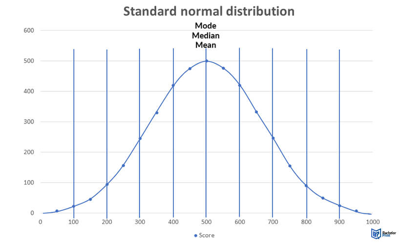
- The mean, mode and median are equal – The mode refers to the most frequently occurring data point in a data distribution. The median is the value that separates the upper from the lower half in an ordered data set. These measures of distribution are equal.

Normal distribution: Empirical rule
The empirical rule, also known as the three-sigma rule or the 68-95-99.7 rule, shows where most of the values fall in a normal distribution:
- Approximately 68% of the values fall between the mean and 1 standard deviation.
- Approximately 95% of the values lie between the mean and 2 standard deviations.
- Around 99.7% of the values fall between the mean and 3 standard deviations.
The empirical rule can be used as a measure of “normality”. If too many data points are outside the three boundaries, then a distribution may not be normal. It can also show the outliers in your data range, i.e. values that are too small or too large, which may affect the shape of the curve.
Normal distribution: Central limit theorem
The central limit theorem postulates that if you have sizeable samples from a given population, the means will be normally distributed even if the population is not necessarily normally distributed. The central limit theorem highlights the following:
- The law of large numbers, which states, as the sample size grows larger, the sample mean moves towards the population mean.
- For several large samples, the mean of the sampling distribution is distributed normally.
The central limit theorem asserts that the assumption of “normality” is unnecessary when conducting parametric tests if the researcher uses a sizeable sample. Parametric tests can be used in large samples of any distribution type as long as the groups have comparable variance and the data in the set is independent.
Formula of the normal curve
A probability density function is used to plot a normal curve after determining the mean and standard deviation. The area under the curve shows the probability, and the total area covered by the curve is equal to 100% or 1, as provided.
Normal Probability density formula:
– Probability
– the value of the variable
– mean
– standard deviation
– variance
Standard normal distribution
The standard normal distribution is a normal distribution with a mean of zero and a standard deviation of 1. The standard normal distribution is also known as the z- distribution, as its observations are denoted with z rather than x. Z-scores in a standard normal distribution show where each value falls away from the mean using the number of standard deviations.
Calculating probability in a z-distribution
Every z-score is assigned a probability (p-value) which shows the probability of the occurrence of some values falling below the z-score.
- ✓ Free express delivery
- ✓ Individual embossing
- ✓ Selection of high-quality bindings
FAQs
The distribution is divisible into two equal halves. It features a peak represented by a curve where values are distributed around a central point.
In a normal distribution, data is not skewed, and the data points form a bell curve. Additionally, the main measures of tendency, i.e. the mean and mode, are similar to the mean.
A z-distribution is commonly known as a standard normal distribution. In a z-distribution, the mean is o, and the standard deviation is 1.
These tests assume that a sample is obtained from a population that exhibits the properties of a normal distribution. They usually focus on comparisons between the variance and the mean.
